Introduction
Welcome to the se-lib User’s Guide with examples. The examples after the User’s Guide can be run separately from their cells, copied and pasted.
Installation
Run the cell below once at the beginning of each session to install the se-lib library. The from selib import * statement will import all its functions and classes to be called with no alias in the notebook.
!pip install -q se-lib

from selib import *
System Dynamics Modeling User’s Guide
Table of Contents
1. Overview
This manual provides an introduction and reference for modeling continuous systems using the se-lib Python package. se-lib supports the construction and simulation of system dynamics models using standard stock and flow structures using both procedural and object-oriented approaches. It adheres to the XMILE standard for system dynamics models and integrates with PySD for simulation execution. Models are compatible with Vensim and iThink/Stella tools using XMILE and MDL formats for importing and exporting.
The object-oriented interface is built around the SystemDynamicsModel class, enabling encapsulation of models, concurrent instantiation, and extensions of the model class. Users may also use the original procedural API for quick prototyping or compatibility with existing scripts. The procedural approach provides a more implicit modeling, but can be less flexible.
The manual includes reusable modeling templates, core system dynamics patterns such as goal-gap control and balancing loops, recommended modeling practices, detailed API documentation, and visual representations of feedback logic. It is suitable for a wide range of applications in systems thinking, behavioral simulation, engineering analysis, and education.
Detailed function references and more examples are available online at http://selib.org/function_reference.html#system-dynamics.
2. Getting Started with SE-Lib
To install the latest version of se-lib, use pip:
pip install se-lib
A system model is described by defining the standard elements for stocks (levels), flows (rates), and auxiliary constants or equations. Utility functions are available for equation formulation, data collection and displaying output.
Model construction begins by importing se-lib and initializing a model with the required time parameters. Simulations operate over a user-defined time horizon and return data as pandas DataFrames, which can be used for analysis and visualization.
from selib import *
init_sd_model(start=0, stop=30, dt=1)
Refer to Section 11 for a complete description of the modeling API.
3. Modeling Guidance and Tips
Modeling with se-lib requires attention to syntax, naming conventions, and logical structure. Names of model elements are specified as character strings and should not contain spaces; underscores (_) must be used to separate terms (e.g., Production_Rate). Variable names are case-sensitive and must exactly match those used in equations.
Equations are expressed as strings using standard arithmetic operators. Variables referenced in equations must already be defined within the model scope. The simulator does not check equations at entry time, so errors from undefined variables or misspellings will only become apparent at runtime.
Conditional statements can be expressed with logical constructs or, and, and not or the XMILE uppercase standards OR, AND, and NOT. The if_then_else(condition, value if true, value if false) or uppercase IF_THEN_ELSE(condition, value if true, value if false) are available.
Random number functions such as random() and random.uniform(a, b) are supported and internally translated into XMILE-compliant expressions. These generate new values at each timestep and are useful for modeling uncertainty or variability in external influences.
Time in se-lib is dimensionless. Modelers must maintain consistency in time unit interpretation (e.g., using all variables in units of days, months, etc.). Inconsistent use of time units can lead to misleading or invalid results.
The draw_model() function is recommended for verifying model structure prior to simulation. This visual representation helps ensure the correctness of stock-flow relationships and the presence of intended feedback loops.
4. Basic Modeling Patterns
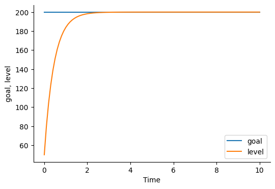
4.1 Negative Feedback Loop
This classic balancing structure adjusts a level toward a target over time. It works by calculating the gap between a goal and the current level, then feeding a corrective flow in the direction that reduces this gap. The delay serves as a time constant, governing the speed of the system’s response. Over time, the level asymptotically approaches the goal value.
from selib import *

# negative feedback
init_sd_model(start=0, stop=5, dt=.1)
add_stock("level", 50, inflows=["rate"])
add_auxiliary("delay", .5)
add_auxiliary("goal", 100)
add_flow("rate", "(goal - level) / delay")

draw_model()
run_model()
plot_graph("level")


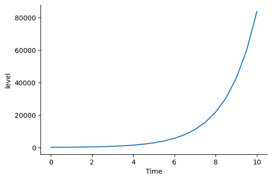
4.2 Exponential Growth
This reinforcing loop demonstrates positive feedback. The flow increases as the stock increases, which in turn further amplifies the flow. This results in exponential behavior and is frequently seen in unchecked population growth, viral spread, or compound interest.
from selib import *

# exponential growth
init_sd_model(start=0, stop=10, dt=.5)
add_stock("level", 100, inflows=["rate"])
add_auxiliary("growth_fraction", .8)
add_flow("rate", "growth_fraction * level")

draw_model()
run_model()
plot_graph('level')


4.3 Balancing Loop
A balancing loop with inventory control adjusts production to maintain a desired stock level. When inventory falls below target, production increases; when it’s above target, production slows. This loop exhibits goal-seeking behavior and helps stabilize system performance. External demand acts as an opposing outflow.
from selib import *

init_sd_model(0, 10, 1)
add_stock("Inventory", 50, inflows=["Production_Rate"], outflows=["Demand_Rate"])
add_auxiliary("Target_Inventory", 100)
add_auxiliary("Adj_Time", 4)
add_flow("Production_Rate", "(Target_Inventory - Inventory) / Adj_Time")
add_auxiliary("Demand", 10)
add_flow("Demand_Rate", "Demand")

draw_model()
run_model()
plot_graph(["Inventory", "Production_Rate"])


4.4 Goal-Gap Structure
This control structure reduces the deviation between a system’s state and a set point. A feedback signal (difference between goal and current value) is amplified by a gain factor and used to drive the stock toward the goal.
from selib import *

init_sd_model(0, 30, 1)
add_stock("Temperature", 20, inflows=["Heating"])
add_auxiliary("Set_Point", 22)
add_auxiliary("Gain", 1.5)
add_flow("Heating", "(Set_Point - Temperature) * Gain")

draw_model()
run_model()
plot_graph(["Temperature", "Set_Point"])


4.5 First-Order Delay
First-order delays represent lagged responses where a stock adjusts toward an input with exponential smoothing. The greater the delay time, the slower the convergence.
from selib import *

init_sd_model(0, 15, 1)
add_stock("Output", 0, inflows=["Flow"])
add_auxiliary("Input", 100)
add_auxiliary("Delay_Time", 5)
add_flow("Flow", "(Input - Output) / Delay_Time")

draw_model()
run_model()
plot_graph(["Input", "Output"])


4.6 Second-Order Delay
A second-order delay structure creates smoother responses by cascading two first-order delays. This is useful when modeling systems with inertia or buffer stages such as material transport, bureaucratic processes, or cognitive recognition lags.
from selib import *

init_sd_model(0, 30, 1)
add_stock("Stage1", 0, inflows=["Flow1"], outflows=["Flow2"])
add_stock("Stage2", 0, inflows=["Flow2"])
add_auxiliary("Input", 100)
add_auxiliary("DelayTime", 5)
add_flow("Flow1", "(Input - Stage1) / DelayTime")
add_flow("Flow2", "(Stage1 - Stage2) / DelayTime")

draw_model()
run_model()
plot_graph(["Stage1", "Stage2"])


…

5. Displaying Output
Upon execution of a system dynamics model, se-lib returns simulation results as a pandas.DataFrame object. This output contains the time-indexed values of all defined stocks, flows, and auxiliaries. The DataFrame facilitates further analysis, visualization, or export to external tools. The `run_model() function will execute a simulation and display a Pandas dataframe of the output. To execute a model and capture its output:
results = run_model()
Each column in the DataFrame corresponds to a model variable, and each row represents a timestep, as defined by the start, stop, and dt parameters provided during model initialization.
To inspect specific variables or values at particular timesteps, standard pandas indexing may be used:
results['Population']               # Full time series for Population
results['Births'][10]              # Value of Births at the 10th timestep
results[['Population', 'Births']] # Multiple variables
This structured output enables direct integration with plotting functions, statistical analysis routines, or export mechanisms. All graphing and saving operations described in Section 6 operate directly on this result structure.
6. Graphing Functions
se-lib provides built-in graphing capabilities to visualize model outputs directly from the simulation results. These graphs are generated using the matplotlib library and support both single-variable and multi-variable plots.
Plotting to Screen
The plot_graph() function displays simulation results interactively. It supports multiple input formats: single variable names, separate arguments, or a list of variables.
plot_graph("Population")
plot_graph("Births", "Deaths")
plot_graph(["Population", "Births", "Deaths"])
When a list is used, variables are plotted together on a shared axis. When passed as separate arguments, they are displayed on individual subplots.
Saving to File
The save_graph() function saves output graphs to image files. The default format is PNG, and the format may be changed by modifying the filename extension.
save_graph("Population", filename="population_plot.png")
save_graph(["Births", "Deaths"], filename="flow_graph.svg")
Saved graphs are rendered as separate figures and written to disk, which is useful for reporting or presentation workflows. As with plotting, graphing functions operate on the output returned by run_model().
7. Random Number Functions
se-lib supports stochastic modeling using random number generation within auxiliary and flow equations. This allows the representation of uncertainty, noise, or nondeterministic behavior in the modeled system. In equations for auxiliaries and rates, the random number functions supported are called as if the following import has occurred: from random import random, random.uniform.
The random functions supported are:
random(): returns a new float uniformly distributed between 0 and 1 at each timestep.random.uniform(min, max): returns a new float uniformly distributed betweenminandmaxat each timestep.
These functions are automatically translated to XMILE-compatible expressions when the model is compiled for simulation. For xmile format compatibility, the functions RANDOM_0_1 and RANDOM_UNIFORM(min, max) are equivalent and also acceptable.
Example
The following example defines an auxiliary variable using random noise:
init_sd_model(start=0, stop=3, dt=.5)
add_auxiliary("random_parameter", "20*random()")
run_model()
( INITIAL TIME FINAL TIME TIME STEP SAVEPER random_parameter
0.0 0 3 0.5 0.5 0.087466
0.5 0 3 0.5 0.5 11.174929
1.0 0 3 0.5 0.5 13.506344
1.5 0 3 0.5 0.5 4.342211
2.0 0 3 0.5 0.5 5.449781
2.5 0 3 0.5 0.5 7.323554
3.0 0 3 0.5 0.5 17.220789,
Each timestep generates a new random value for Stochastic_Input, producing a non-repeating time series. It is important to note that random values are recomputed each time the model is run, and results may vary unless reproducibility measures (e.g., seeding) are implemented outside SE-Lib.
8. Utility and Test Functions
Standard test functions are available for pulse, ramp and step inputs as shown below. The full set of functions available in PySD can be used but have not all been tested.
init_sd_model(0, 10, 1)
add_stock("Level", 0, inflows=["Pulse", "Ramp"])
add_flow("Pulse", "pulse(100, 2)")
add_flow("Ramp", "ramp(3, 5)")
run_model()
plot_graph("Pulse", "Ramp", "Level")
9. Advanced Usage
9.1 Extending a Model Instance
Create a new class that extends a population model by adding carrying capacity with the following.
class PopulationWithCapacityModel(SystemDynamicsModel):
    def __init__(self, start, stop, dt, initial_population, carrying_capacity):
        super().__init__(start, stop, dt)
        self.add_stock("Population", initial=initial_population, inflows=["Births"], outflows=["Deaths"])
        self.add_auxiliary("BirthRate", equation=0.02)
        self.add_auxiliary("CarryingCapacity", equation=carrying_capacity)
        self.add_auxiliary("CrowdingEffect", equation="Population / CarryingCapacity")
        self.add_auxiliary("EffectiveGrowthRate", equation="BirthRate * (1 - CrowdingEffect)")
        self.add_flow("Births", equation="Population * EffectiveGrowthRate")
        self.add_auxiliary("DeathRate", equation=0.01)
        self.add_flow("Deaths", equation="Population * DeathRate") # Keep a simple death rate

# Create an instance of the extended model
population_capacity_model = PopulationWithCapacityModel(start=0, stop=200, dt=1, initial_population=50, carrying_capacity=500)
9.1 PySD Integration
SE-Lib is fully compatible with PySD. Any PySD function or supported XMILE structure may be used where appropriate. See PySD Docs for advanced formulations.
10. Appendix A - Function Reference
The following functions and methods define the modeling API for se-lib. All functions can be used in either procedural or object-oriented workflows.
init_sd_model(start, stop, dt, stop_when=None)
Initializes a new system dynamics model over the specified simulation time frame.
Args: - start (float): Start time of the simulation. - stop (float): End time of the simulation. - dt (float): Time step for numerical integration. - stop_when (float): Logical condition using model variables to stop the simulation.
Returns: - SystemDynamicsModel instance
Example:
init_sd_model(start=0, stop=50, dt=1.0)
Examples with stop_when:
init_sd_model(start=0, stop=50, dt=1.0, stop_when("stock1 >= 100")
init_sd_model(start=0, stop=50, dt=1.0, stop_when("stock1 >= 100 or stock2 >=80")
add_stock(name, initial, inflows=[], outflows=[])
Adds a stock variable (level) to the system dynamics model.
Args: - name (str): Name of the stock. - initial (float): Initial value of the stock. - inflows (list, optional): Names of inflow variables affecting this stock. - outflows (list, optional): Names of outflow variables affecting this stock.
Returns: - None
Example:
add_stock("Population", initial=100, inflows=["Births"], outflows=["Deaths"])
add_flow(name, equation)
Defines a flow (rate of change) for use in stock updates.
Args: - name (str): Name of the flow. - equation (str): Equation as a string to compute the flow value.
Returns: - None
Example:
add_flow("Births", "Birth_Rate * Population")
add_auxiliary(name, equation)
Defines an auxiliary variable or constant used in the model.
Args: - name (str): Name of the auxiliary variable. - equation (str): String representation of the equation or constant value.
Returns: - None
Example:
add_auxiliary("Birth_Rate", "0.02")
add_auxiliary_lookup(name, input, xpoints, ypoints)
Creates a lookup function for a nonlinear relationship.
Args: - name (str): Name of the auxiliary variable. - input (str): Name of the input variable used in the lookup. - xpoints (list): List of input values (x-axis). - ypoints (list): List of output values (y-axis).
Returns: - None
Example:
add_auxiliary_lookup("Saturation", "Population", [0, 1000, 2000], [1, 0.5, 0.1])
plot_graph(*outputs)
Plots model results using matplotlib.
Args: - *outputs (str or list): Names of variables to plot (e.g., “Population”, [“Births”, “Deaths”]).
Returns: - None
Example:
plot_graph("Population")
plot_graph(["Births", "Deaths"])
save_graph(*outputs, filename='graph.png')
Saves a plot of the simulation
draw_sd_model(filename=None, format=’svg’)
Generates and renders a visual system dynamics model diagram using Graphviz.
get_stop_time()
Returns the logical end time based on a stop_when condition.
get_model_structure()
Returns a dictionary of model components (stocks, flows, auxiliaries).
Examples
Exponential Growth
from selib import *

# exponential_growth
init_sd_model(start=0, stop=10, dt=.5)
add_stock("level", 100, inflows=["rate"])
add_auxiliary("growth_fraction", .8)
add_flow("rate", "growth_fraction * level")

draw_model()
run_model()

save_graph('level', filename="exponential_growth.png")
--------------

      INITIAL TIME  FINAL TIME  TIME STEP  SAVEPER  growth_fraction  \
time
0.0              0          10        0.5      0.5              0.8
0.5              0          10        0.5      0.5              0.8
1.0              0          10        0.5      0.5              0.8
1.5              0          10        0.5      0.5              0.8
2.0              0          10        0.5      0.5              0.8
2.5              0          10        0.5      0.5              0.8
3.0              0          10        0.5      0.5              0.8
3.5              0          10        0.5      0.5              0.8
4.0              0          10        0.5      0.5              0.8
4.5              0          10        0.5      0.5              0.8
5.0              0          10        0.5      0.5              0.8
5.5              0          10        0.5      0.5              0.8
6.0              0          10        0.5      0.5              0.8
6.5              0          10        0.5      0.5              0.8
7.0              0          10        0.5      0.5              0.8
7.5              0          10        0.5      0.5              0.8
8.0              0          10        0.5      0.5              0.8
8.5              0          10        0.5      0.5              0.8
9.0              0          10        0.5      0.5              0.8
9.5              0          10        0.5      0.5              0.8
10.0             0          10        0.5      0.5              0.8

              rate         level
time
0.0      80.000000    100.000000
0.5     112.000000    140.000000
1.0     156.800000    196.000000
1.5     219.520000    274.400000
2.0     307.328000    384.160000
2.5     430.259200    537.824000
3.0     602.362880    752.953600
3.5     843.308032   1054.135040
4.0    1180.631245   1475.789056
4.5    1652.883743   2066.104678
5.0    2314.037240   2892.546550
5.5    3239.652136   4049.565170
6.0    4535.512990   5669.391238
6.5    6349.718186   7937.147733
7.0    8889.605460  11112.006826
7.5   12445.447645  15556.809556
8.0   17423.626702  21779.533378
8.5   24393.077383  30491.346729
9.0   34150.308337  42687.885421
9.5   47810.431672  59763.039589
10.0  66934.604340  83668.255425
--------------
Negative Feedback
# negative feedback
from selib import *

init_sd_model(start=0, stop=10, dt=.1)
add_stock("level", 50, inflows=["rate"])
add_auxiliary("delay", .5)
add_auxiliary("goal", 100)
add_flow("rate", "(goal - level) / delay")

draw_model()
run_model()

save_graph(['level', 'goal', 'rate'], filename="negative_feedback.svg")
--------------

      INITIAL TIME  FINAL TIME  TIME STEP  SAVEPER  delay  goal          rate  \
time
0.0              0          10        0.1      0.1    0.5   100  1.000000e+02
0.1              0          10        0.1      0.1    0.5   100  8.000000e+01
0.2              0          10        0.1      0.1    0.5   100  6.400000e+01
0.3              0          10        0.1      0.1    0.5   100  5.120000e+01
0.4              0          10        0.1      0.1    0.5   100  4.096000e+01
...            ...         ...        ...      ...    ...   ...           ...
9.6              0          10        0.1      0.1    0.5   100  4.973231e-08
9.7              0          10        0.1      0.1    0.5   100  3.978585e-08
9.8              0          10        0.1      0.1    0.5   100  3.182868e-08
9.9              0          10        0.1      0.1    0.5   100  2.546295e-08
10.0             0          10        0.1      0.1    0.5   100  2.037035e-08

       level
time
0.0    50.00
0.1    60.00
0.2    68.00
0.3    74.40
0.4    79.52
...      ...
9.6   100.00
9.7   100.00
9.8   100.00
9.9   100.00
10.0  100.00

[101 rows x 8 columns]
--------------

Goal Seeking Behavior
from selib import *

# goal seeking behavior with negative feedback

init_sd_model(start=0, stop=10, dt=.1)
add_stock("level", 50, inflows=["rate"])
add_auxiliary("time_constant", .5)
add_auxiliary("goal", 200)
add_flow("rate", "(goal - level) / time_constant")

draw_model()
run_model()

plot_graph(['goal', 'level'])
--------------

      INITIAL TIME  FINAL TIME  TIME STEP  SAVEPER  time_constant  goal  \
time
0.0              0          10        0.1      0.1            0.5   200
0.1              0          10        0.1      0.1            0.5   200
0.2              0          10        0.1      0.1            0.5   200
0.3              0          10        0.1      0.1            0.5   200
0.4              0          10        0.1      0.1            0.5   200
...            ...         ...        ...      ...            ...   ...
9.6              0          10        0.1      0.1            0.5   200
9.7              0          10        0.1      0.1            0.5   200
9.8              0          10        0.1      0.1            0.5   200
9.9              0          10        0.1      0.1            0.5   200
10.0             0          10        0.1      0.1            0.5   200

              rate   level
time
0.0   3.000000e+02   50.00
0.1   2.400000e+02   80.00
0.2   1.920000e+02  104.00
0.3   1.536000e+02  123.20
0.4   1.228800e+02  138.56
...            ...     ...
9.6   1.491970e-07  200.00
9.7   1.193576e-07  200.00
9.8   9.548609e-08  200.00
9.9   7.638886e-08  200.00
10.0  6.111111e-08  200.00

[101 rows x 8 columns]
--------------
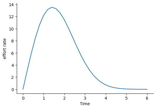
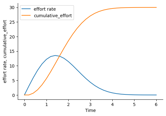
Rayleigh Curve Staffing
# Rayleigh Curve Staffing
from selib import *

init_sd_model(start=0, stop=6, dt=.2)
add_stock("cumulative_effort", 0, inflows=["effort rate"])
add_flow("effort rate",
         "learning_function * (estimated_total_effort - cumulative_effort)")
add_auxiliary("learning_function", "manpower_buildup_parameter * time")
add_auxiliary("manpower_buildup_parameter", .5)
add_auxiliary("estimated_total_effort", 30)

draw_model()
run_model()

save_graph("effort rate", filename="rayleigh_curve_effort_rate.png")
save_graph(["effort rate", "cumulative_effort"],
           filename="rayleigh_curve_components.png")
--------------

      INITIAL TIME  FINAL TIME  TIME STEP  SAVEPER  learning_function  \
time
0.0              0           6        0.2      0.2                0.0
0.2              0           6        0.2      0.2                0.1
0.4              0           6        0.2      0.2                0.2
0.6              0           6        0.2      0.2                0.3
0.8              0           6        0.2      0.2                0.4
1.0              0           6        0.2      0.2                0.5
1.2              0           6        0.2      0.2                0.6
1.4              0           6        0.2      0.2                0.7
1.6              0           6        0.2      0.2                0.8
1.8              0           6        0.2      0.2                0.9
2.0              0           6        0.2      0.2                1.0
2.2              0           6        0.2      0.2                1.1
2.4              0           6        0.2      0.2                1.2
2.6              0           6        0.2      0.2                1.3
2.8              0           6        0.2      0.2                1.4
3.0              0           6        0.2      0.2                1.5
3.2              0           6        0.2      0.2                1.6
3.4              0           6        0.2      0.2                1.7
3.6              0           6        0.2      0.2                1.8
3.8              0           6        0.2      0.2                1.9
4.0              0           6        0.2      0.2                2.0
4.2              0           6        0.2      0.2                2.1
4.4              0           6        0.2      0.2                2.2
4.6              0           6        0.2      0.2                2.3
4.8              0           6        0.2      0.2                2.4
5.0              0           6        0.2      0.2                2.5
5.2              0           6        0.2      0.2                2.6
5.4              0           6        0.2      0.2                2.7
5.6              0           6        0.2      0.2                2.8
5.8              0           6        0.2      0.2                2.9
6.0              0           6        0.2      0.2                3.0

      manpower_buildup_parameter  estimated_total_effort  effort rate  \
time
0.0                          0.5                      30     0.000000
0.2                          0.5                      30     3.000000
0.4                          0.5                      30     5.880000
0.6                          0.5                      30     8.467200
0.8                          0.5                      30    10.612224
1.0                          0.5                      30    12.204058
1.2                          0.5                      30    13.180382
1.4                          0.5                      30    13.531859
1.6                          0.5                      30    13.299884
1.8                          0.5                      30    12.568391
2.0                          0.5                      30    11.451200
2.2                          0.5                      30    10.077056
2.4                          0.5                      30     8.574659
2.6                          0.5                      30     7.059802
2.8                          0.5                      30     5.626120
3.0                          0.5                      30     4.340149
3.2                          0.5                      30     3.240645
3.4                          0.5                      30     2.341366
3.6                          0.5                      30     1.636202
3.8                          0.5                      30     1.105345
4.0                          0.5                      30     0.721383
4.2                          0.5                      30     0.454471
4.4                          0.5                      30     0.276145
4.6                          0.5                      30     0.161671
4.8                          0.5                      30     0.091098
5.0                          0.5                      30     0.049345
5.2                          0.5                      30     0.025659
5.4                          0.5                      30     0.012790
5.6                          0.5                      30     0.006101
5.8                          0.5                      30     0.002780
6.0                          0.5                      30     0.001208

      cumulative_effort
time
0.0            0.000000
0.2            0.000000
0.4            0.600000
0.6            1.776000
0.8            3.469440
1.0            5.591885
1.2            8.032696
1.4           10.668773
1.6           13.375145
1.8           16.035121
2.0           18.548800
2.2           20.839040
2.4           22.854451
2.6           24.569383
2.8           25.981343
3.0           27.106567
3.2           27.974597
3.4           28.622726
3.6           29.090999
3.8           29.418239
4.0           29.639308
4.2           29.783585
4.4           29.874479
4.6           29.929708
4.8           29.962043
5.0           29.980262
5.2           29.990131
5.4           29.995263
5.6           29.997821
5.8           29.999041
6.0           29.999597
--------------
--------------
Random Functions and Measuring Stop Time
This example illustrates measuring elapsed simulation time using the stop_when initialization parameter and get_stop_time() function. It captures the project end when staffing effort rate goes to zero.
from selib import *

init_sd_model(start=0, stop=6, dt=.2, stop_when="effort_rate <= 0")
add_stock("cumulative_effort", 0, inflows=["effort rate"])
add_flow("effort_rate",
    "learning_function * (estimated_total_effort - cumulative_effort)")
add_auxiliary("learning_function", "manpower_buildup_parameter * time")
add_auxiliary("manpower_buildup_parameter", 'random.uniform(.2, .7)')
add_auxiliary("estimated_total_effort", 'random.uniform(25, 35)')

run_model()

print(f"Project end time is {get_stop_time()}")
Simulation ends at time = 3.0
      INITIAL TIME  FINAL TIME  TIME STEP  SAVEPER  learning_function  \
time
0.0              0           6        0.2      0.2           0.000000
0.2              0           6        0.2      0.2           0.122395
0.4              0           6        0.2      0.2           0.235581
0.6              0           6        0.2      0.2           0.206761
0.8              0           6        0.2      0.2           0.304143
1.0              0           6        0.2      0.2           0.207023
1.2              0           6        0.2      0.2           0.459536
1.4              0           6        0.2      0.2           0.320776
1.6              0           6        0.2      0.2           0.781662
1.8              0           6        0.2      0.2           0.851055
2.0              0           6        0.2      0.2           1.260378
2.2              0           6        0.2      0.2           1.045175
2.4              0           6        0.2      0.2           1.072665
2.6              0           6        0.2      0.2           1.511612
2.8              0           6        0.2      0.2           1.299925
3.0              0           6        0.2      0.2           1.825976

      manpower_buildup_parameter  estimated_total_effort  effort_rate  \
time
0.0                     0.682189               34.323998     0.000000
0.2                     0.611974               27.620483     3.380603
0.4                     0.588953               30.330142     6.985926
0.6                     0.344601               29.166838     5.601875
0.8                     0.380179               33.010074     9.068448
1.0                     0.207023               31.018010     5.384799
1.2                     0.382947               32.624585    12.196203
1.4                     0.229126               28.600847     6.440316
1.6                     0.488538               30.481037    16.156478
1.8                     0.472808               29.680247    14.159276
2.0                     0.630189               31.585909    19.801960
2.2                     0.475079               25.422697     5.839935
2.4                     0.446944               31.348129    11.096682
2.6                     0.581389               29.838478    10.000791
2.8                     0.464259               30.166600     6.426755
3.0                     0.608659               25.307849    -2.191463

      cumulative_effort
time
0.0            0.000000
0.2            0.000000
0.4            0.676121
0.6            2.073306
0.8            3.193681
1.0            5.007370
1.2            6.084330
1.4            8.523571
1.6            9.811634
1.8           13.042930
2.0           15.874785
2.2           19.835177
2.4           21.003164
2.6           23.222500
2.8           25.222658
3.0           26.508009
Project end time is 3.0
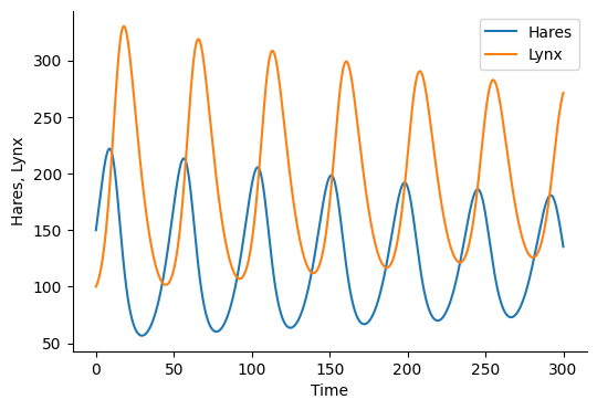
Predator Prey Model
# Predator Prey Model with Carrying Capacity
import selib as se

# Initialize model
init_sd_model(start=0, stop=300, dt=0.25)

# Auxiliaries
add_auxiliary_lookup("Carrying_Capacity_Effect", "Hares",
                     ["0, 500, 1000, 1500, 2000"], ["1, .8, .5, .2, .05"])

add_auxiliary("Hare_Growth_Rate", "0.162 * Carrying_Capacity_Effect")
add_auxiliary("Hare_Death_Rate", ".0008 * Lynx")
add_auxiliary("Lynx_Death_Rate", "0.12")
add_auxiliary("Lynx_Birth_Rate", "0.001 * Hares")

# Stocks
add_stock("Hares", "150", inflows=["Hare_Births"], outflows=["Hare_Deaths"])
add_stock("Lynx", "100", inflows=["Lynx_Births"], outflows=["Lynx_Deaths"])

# Flows
add_flow("Hare_Births", "Hare_Growth_Rate * Hares")
add_flow("Hare_Deaths", "Hare_Death_Rate * Hares")
add_flow("Lynx_Births", "Lynx_Birth_Rate * Lynx")
add_flow("Lynx_Deaths", "Lynx_Death_Rate * Lynx")

d = draw_model_diagram(filename="sd")
results = run_model()
save_graph(["Hares", "Lynx"])
--------------

        INITIAL TIME  FINAL TIME  TIME STEP  SAVEPER  \
time
0.00               0         300       0.25     0.25
0.25               0         300       0.25     0.25
0.50               0         300       0.25     0.25
0.75               0         300       0.25     0.25
1.00               0         300       0.25     0.25
...              ...         ...        ...      ...
299.00             0         300       0.25     0.25
299.25             0         300       0.25     0.25
299.50             0         300       0.25     0.25
299.75             0         300       0.25     0.25
300.00             0         300       0.25     0.25

        Carrying_Capacity_Effect  Hare_Growth_Rate  Hare_Death_Rate  \
time
0.00                    0.940000          0.152280         0.080000
0.25                    0.938916          0.152104         0.080600
0.50                    0.937824          0.151927         0.081259
0.75                    0.936725          0.151750         0.081979
1.00                    0.935622          0.151571         0.082762
...                          ...               ...              ...
299.00                  0.942403          0.152669         0.212617
299.25                  0.943266          0.152809         0.213893
299.50                  0.944132          0.152949         0.215060
299.75                  0.945000          0.153090         0.216118
300.00                  0.945866          0.153230         0.217063

        Lynx_Death_Rate  Lynx_Birth_Rate  Hare_Births  Hare_Deaths  \
time
0.00               0.12         0.150000    22.842000    12.000000
0.25               0.12         0.152710    23.227933    12.308466
0.50               0.12         0.155440    23.615661    12.630947
0.75               0.12         0.158187    24.004731    12.967987
1.00               0.12         0.160946    24.394660    13.320143
...                 ...              ...          ...          ...
299.00             0.12         0.143993    21.983347    30.615492
299.25             0.12         0.141835    21.673716    30.337545
299.50             0.12         0.139669    21.362341    30.037341
299.75             0.12         0.137501    21.049955    29.716338
300.00             0.12         0.135334    20.737271    29.376063

        Lynx_Births  Lynx_Deaths       Hares        Lynx
time
0.00      15.000000    12.000000  150.000000  100.000000
0.25      15.385583    12.090000  152.710500  100.750000
0.50      15.788684    12.188867  155.440367  101.573896
0.75      16.209984    12.296862  158.186545  102.473850
1.00      16.650179    12.414256  160.945731  103.452130
...             ...          ...         ...         ...
299.00    38.269365    31.892621  143.993301  265.771845
299.25    37.921932    32.083924  141.835264  267.366031
299.50    37.546676    32.259064  139.669307  268.825533
299.75    37.145423    32.417692  137.500557  270.147436
300.00    36.720078    32.559524  135.333961  271.329369

[1201 rows x 15 columns]
--------------
# patch to increase padding for model diagrams
import graphviz

# Store original methods
_original_digraph_init = graphviz.Digraph.__init__

def patched_digraph_init(self, *args, **kwargs):
    _original_digraph_init(self, *args, **kwargs)
    # Apply defaults
    self.attr('graph', pad='1')

# Apply patches
graphviz.Digraph.__init__ = patched_digraph_init
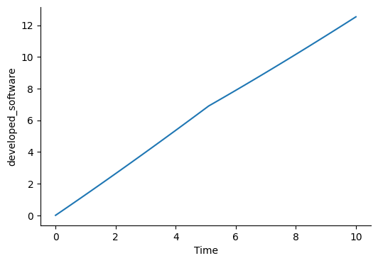
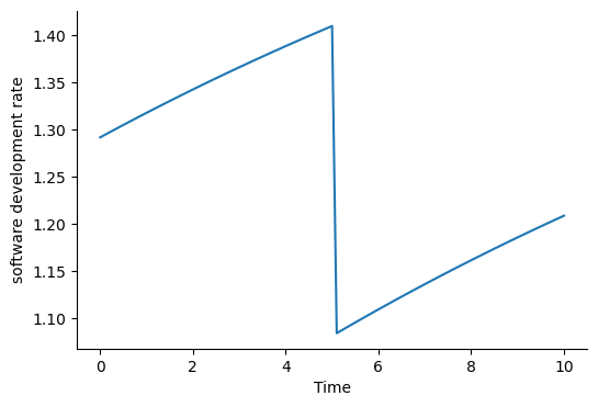
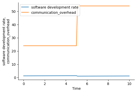
Brooks’s Law Model
# Brooks's Law Model
from selib import *
init_sd_model(start=0, stop=10, dt=.1)
add_stock("requirements", 500, inflows=[], outflows=["software development rate"])
add_stock("developed_software", 0, inflows=["software development rate"])
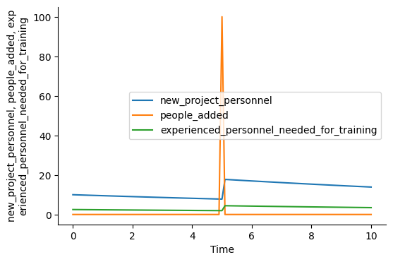
add_flow("software development rate", "nominal_productivity*(1.-communication_overhead/100.)*(.8*new_project_personnel+1.2*(experienced_personnel-experienced_personnel_needed_for_training))")
add_stock("experienced_personnel", 10.0, inflows=["assimilation rate"])
add_stock("new_project_personnel", 10.0, inflows=["people_added"], outflows=["assimilation rate"])
add_flow("assimilation rate", "new_project_personnel/20")
add_flow("people_added", "pulse(10,5)")
add_auxiliary("nominal_productivity", .1)
add_auxiliary("training_overhead_FTE_experienced", 25.)
add_auxiliary("experienced_personnel_needed_for_training", "new_project_personnel*training_overhead_FTE_experienced/100.")
add_auxiliary_lookup("communication_overhead", "experienced_personnel + new_project_personnel",
["0, 5, 10, 15, 20, 25, 30"], ["0, 1.5, 6, 13.5, 24, 37.5, 54"])
draw_sd_model()
output = run_model()
plot_graph("developed_software")
plot_graph("software development rate")
plot_graph(["software development rate", "communication_overhead"])
plot_graph(["new_project_personnel", "people_added", "experienced_personnel_needed_for_training"])
--------------

      INITIAL TIME  FINAL TIME  TIME STEP  SAVEPER  nominal_productivity  \
time
0.0              0          10        0.1      0.1                   0.1
0.1              0          10        0.1      0.1                   0.1
0.2              0          10        0.1      0.1                   0.1
0.3              0          10        0.1      0.1                   0.1
0.4              0          10        0.1      0.1                   0.1
...            ...         ...        ...      ...                   ...
9.6              0          10        0.1      0.1                   0.1
9.7              0          10        0.1      0.1                   0.1
9.8              0          10        0.1      0.1                   0.1
9.9              0          10        0.1      0.1                   0.1
10.0             0          10        0.1      0.1                   0.1

      training_overhead_FTE_experienced  \
time
0.0                                25.0
0.1                                25.0
0.2                                25.0
0.3                                25.0
0.4                                25.0
...                                 ...
9.6                                25.0
9.7                                25.0
9.8                                25.0
9.9                                25.0
10.0                               25.0

      experienced_personnel_needed_for_training  communication_overhead  \
time
0.0                                    2.500000                    24.0
0.1                                    2.487500                    24.0
0.2                                    2.475062                    24.0
0.3                                    2.462687                    24.0
0.4                                    2.450374                    24.0
...                                         ...                     ...
9.6                                    3.540261                    54.0
9.7                                    3.522560                    54.0
9.8                                    3.504947                    54.0
9.9                                    3.487422                    54.0
10.0                                   3.469985                    54.0

      software development rate  assimilation rate  people_added  \
time
0.0                    1.292000           0.500000           0.0
0.1                    1.294660           0.497500           0.0
0.2                    1.297307           0.495012           0.0
0.3                    1.299940           0.492537           0.0
0.4                    1.302560           0.490075           0.0
...                         ...                ...           ...
9.6                    1.200014           0.708052           0.0
9.7                    1.202294           0.704512           0.0
9.8                    1.204563           0.700989           0.0
9.9                    1.206820           0.697484           0.0
10.0                   1.209066           0.693997           0.0

      requirements  developed_software  experienced_personnel  \
time
0.0     500.000000            0.000000              10.000000
0.1     499.870800            0.129200              10.050000
0.2     499.741334            0.258666              10.099750
0.3     499.611603            0.388397              10.149251
0.4     499.481609            0.518391              10.198505
...            ...                 ...                    ...
9.6     487.953319           12.046681              15.838955
9.7     487.833317           12.166683              15.909760
9.8     487.713088           12.286912              15.980211
9.9     487.592632           12.407368              16.050310
10.0    487.471950           12.528050              16.120059

      new_project_personnel
time
0.0               10.000000
0.1                9.950000
0.2                9.900250
0.3                9.850749
0.4                9.801495
...                     ...
9.6               14.161045
9.7               14.090240
9.8               14.019789
9.9               13.949690
10.0              13.879941

[101 rows x 15 columns]
--------------
--------------
--------------
--------------
--------------
Object Oriented Simulation Using Classes
# @title Capability Development Model with Stop Condition
from selib import *
# Initialize SystemDynamicsModel model instance
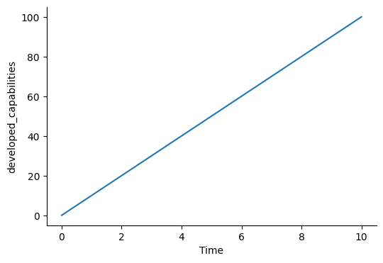
model = SystemDynamicsModel(start=0, stop=25, dt=0.1, stop_when="developed_capabilities >= 100")
model.add_stock(name="capabilities_to_do", initial=100, outflows=["development_rate"])
model.add_stock(name="developed_capabilities", initial=0, inflows=["development_rate"])
model.add_flow(name="development_rate", equation="IF capabilities_to_do > 0 THEN 10 ELSE 0")
# Draw the model diagram
model.draw_model()
# Run the model simulation
results = model.run_model()
# Plot the 'developed_capabilities'
model.plot_graph('developed_capabilities')
# Print the stop time
stop_time = model.get_stop_time()
print(f'stop time = {stop_time}')
--------------

Simulation ends at time = 10.0
      INITIAL TIME  FINAL TIME  TIME STEP  SAVEPER  development_rate  \
time
0.0              0          25        0.1      0.1                10
0.1              0          25        0.1      0.1                10
0.2              0          25        0.1      0.1                10
0.3              0          25        0.1      0.1                10
0.4              0          25        0.1      0.1                10
...            ...         ...        ...      ...               ...
9.6              0          25        0.1      0.1                10
9.7              0          25        0.1      0.1                10
9.8              0          25        0.1      0.1                10
9.9              0          25        0.1      0.1                10
10.0             0          25        0.1      0.1                 0

      capabilities_to_do  developed_capabilities
time
0.0                100.0                     0.0
0.1                 99.0                     1.0
0.2                 98.0                     2.0
0.3                 97.0                     3.0
0.4                 96.0                     4.0
...                  ...                     ...
9.6                  4.0                    96.0
9.7                  3.0                    97.0
9.8                  2.0                    98.0
9.9                  1.0                    99.0
10.0                 0.0                   100.0

[101 rows x 7 columns]
--------------
stop time = 10.0
Monte Carlo Simulation and Output Analysis
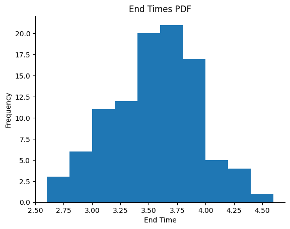
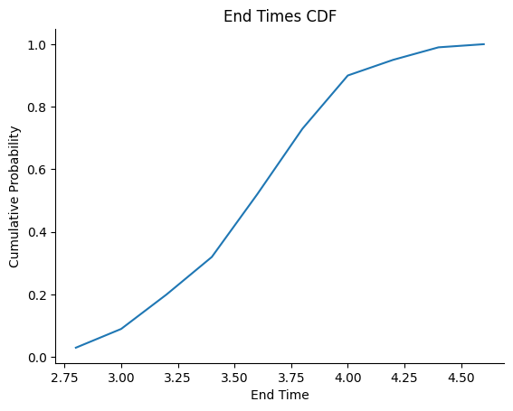
# Monte Carlo simulation for Rayleigh Curve Staffing and end time output analysis
from selib import *
import numpy as np

number_runs = 100

# vary manpower_buildup_parameter and estimated_total_effort in model definition

end_times = []  # initialize output data list

for run in range(number_runs):
    init_sd_model(start=0, stop=6, dt=.2, stop_when="effort_rate <=0")
    add_stock("cumulative_effort", 0, inflows=["effort rate"])
    add_flow(
        "effort_rate",
        "learning_function * (estimated_total_effort - cumulative_effort)")
    add_auxiliary("learning_function", "manpower_buildup_parameter * time")
    add_auxiliary("manpower_buildup_parameter", 'random.uniform(.2, .7)')
    add_auxiliary("estimated_total_effort", f'random.uniform(25, 35)')

    run_model(verbose=False)
    end_times.append(get_stop_time())

print(f'End Time Mean for {number_runs} runs = ', np.mean(end_times))

# PDF histogram with Matplotlib
fig, axis = plt.subplots()
axis.hist(end_times)
axis.set(title=f'End Times PDF', xlabel='End Time', ylabel='Frequency')
plt.savefig(f"end_times_PDF")

# CDF with NumPy and Matplotlib
fig, axis = plt.subplots()
# Use the histogram function to bin the data
histogram_bin_counts, bin_edges = np.histogram (end_times, density=True)
cdf = np.cumsum (histogram_bin_counts)
axis.plot (bin_edges[1:], cdf/cdf[-1])
axis.set(title=f'End Times CDF', xlabel='End Time', ylabel='Cumulative Probability')
plt.savefig(f"end_times_CDF")
End Time Mean for 100 runs = 3.4560000000000004
--------------
--------------
Special Functions
from selib import *

init_sd_model(start=0, stop=6, dt=.2, stop_when="effort_rate <= 0")
add_stock("cumulative_effort", 0, inflows=["effort rate"])
add_flow("effort_rate",
    "learning_function * (estimated_total_effort - cumulative_effort)")
add_auxiliary("learning_function", "manpower_buildup_parameter * time")
add_auxiliary("manpower_buildup_parameter", 'random.uniform(.2, .7)')
add_auxiliary("estimated_total_effort", 'random.uniform(25, 35)')

run_model()

print(f"Project end time is {get_stop_time()}")
Stop When Condition
# demonstrate stop_when condition to end simulation and the get_stop function
# collect time when the stock reaches zero

from selib import *
init_sd_model(start=0, stop=10, dt=.5, stop_when="stock <= 0")
add_stock("stock", 50, outflows=["outflow_rate"])
add_flow("outflow_rate", "20")

run_model()

print('stop time = ', get_stop_time())
Simulation ends at time = 2.5
      INITIAL TIME  FINAL TIME  TIME STEP  SAVEPER  outflow_rate  stock
time
0.0              0          10        0.5      0.5            20   50.0
0.5              0          10        0.5      0.5            20   40.0
1.0              0          10        0.5      0.5            20   30.0
1.5              0          10        0.5      0.5            20   20.0
2.0              0          10        0.5      0.5            20   10.0
2.5              0          10        0.5      0.5            20    0.0
stop time = 2.5
If Then Else
# demonstrate if then else function

from selib import *
init_sd_model(start=0, stop=5, dt=1)

# set conditional variable
# if time > 2 then 1 else 0
add_auxiliary("conditional", "if_then_else(time > 2, 1, 0)")
add_auxiliary("conditional2", "if_then_else(time < 4, .5, .7)")
run_model()
      INITIAL TIME  FINAL TIME  TIME STEP  SAVEPER  conditional  conditional2
time
0                0           5          1        1            0           0.5
1                0           5          1        1            0           0.5
2                0           5          1        1            0           0.5
3                0           5          1        1            1           0.5
4                0           5          1        1            1           0.7
5                0           5          1        1            1           0.7